⚡ Saturday ML Sparks – Linear Regression on Real Data 🧠📊

Linear Regression is one of the most fundamental algorithms in machine learning.

It’s used to model the relationship between a dependent variable (the target) and one or more independent variables (the features).

In this post, we’ll explore how to apply Linear Regression to a real-world dataset and interpret its performance.

---

What Is Linear Regression?

Linear Regression attempts to fit a straight line (or hyperplane in higher dimensions) that best describes the relationship between features and the target.

Mathematically, it follows the equation:

y = β_0 + β_1x_1 + β_2x_2 + … + β_nx_n

Where:

• y → predicted value
• β_0 → intercept
• β_1, β_2, … β_n → coefficients for each feature
• x_1, x_2, … x_n → feature values

The goal is to minimize the Mean Squared Error (MSE) between predicted and actual values.

---

Dataset and Setup

We’ll use the California Housing dataset — a popular regression dataset that predicts median house value based on features such as income, house age, and population.

In case of connectivity or SSL issues, we’ll fall back to the Diabetes dataset, which is included locally with scikit-learn.

from sklearn.datasets import fetch_california_housing, load_diabetes
import pandas as pd

try:
    data = fetch_california_housing(as_frame=True)
    df = data.frame
    target_col = "MedHouseVal"
    print("Using California Housing dataset.")
except Exception:
    data = load_diabetes(as_frame=True)
    df = pd.concat([data.data, data.target.rename("target")], axis=1)
    target_col = "target"
    print("Using Diabetes dataset (fallback).")

This ensures the script works seamlessly both online and offline.

---

Building and Training the Model

We split the data into training and testing sets and fit a Linear Regression model.

from sklearn.model_selection import train_test_split
from sklearn.linear_model import LinearRegression

X = df.drop(columns=[target_col])
y = df[target_col]

X_train, X_test, y_train, y_test = train_test_split(X, y, test_size=0.2, random_state=42)

model = LinearRegression()
model.fit(X_train, y_train)

The model learns a set of coefficients (β) that define how each feature contributes to the prediction.

---

Evaluating Model Performance

Once trained, we evaluate how well the model generalizes to unseen data using Mean Squared Error (MSE) and R² Score.

from sklearn.metrics import mean_squared_error, r2_score

y_pred = model.predict(X_test)

mse = mean_squared_error(y_test, y_pred)
r2 = r2_score(y_test, y_pred)

print(f"Mean Squared Error: {mse:.2f}")
print(f"R² Score: {r2:.2f}")

• MSE measures average squared differences between predictions and actual values. Lower is better.
• R² (Coefficient of Determination) shows how much variance in the target is explained by the features. Closer to 1 indicates a better fit.

---

Visualizing Predictions

A scatter plot of actual vs predicted values helps visualize model accuracy.

Points lying close to the diagonal line indicate strong predictive performance.

import matplotlib.pyplot as plt

plt.figure(figsize=(8, 6))
plt.scatter(y_test, y_pred, alpha=0.5, color='teal')
plt.xlabel("Actual Values")
plt.ylabel("Predicted Values")
plt.title("Actual vs Predicted – Linear Regression")
plt.plot([0, 5], [0, 5], color="orange", linestyle="--")
plt.grid(True, alpha=0.3)
plt.show()

---

Sample Output

The resulting plot looks like this:

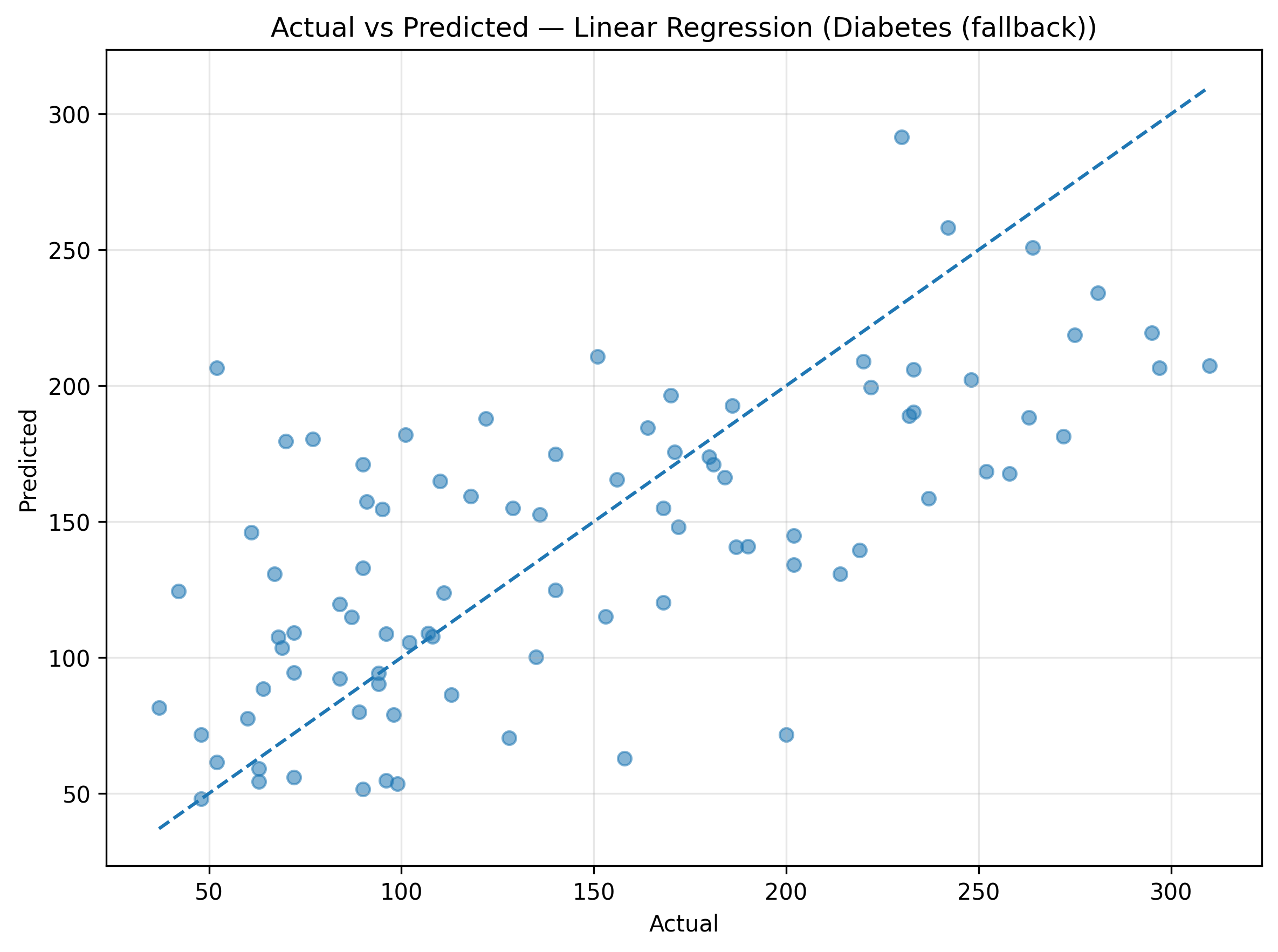
Figure: Actual vs Predicted – Linear Regression.

---

Interpreting the Results

• Good Fit: Points closely align along the diagonal line.
• Underfitting: High MSE, low R² — model is too simple or lacks features.
• Overfitting: Perfect fit on training data but poor generalization on test data — consider regularization or feature reduction.

Even with its simplicity, Linear Regression remains one of the most useful baselines for regression tasks.

---

Key Takeaways

• Linear Regression models the linear relationship between features and a continuous target.
• Use MSE and R² to measure performance.
• Always visualize predictions to spot anomalies or bias.
• For larger or non-linear datasets, consider extensions such as Ridge, Lasso, or Polynomial Regression.

---

Conclusion

Linear Regression is the foundation of many predictive modeling techniques.

By learning to train, evaluate, and interpret such models, you gain essential skills for tackling more advanced machine learning problems.

Start simple — and let the data guide your next steps.

---

Full Script

The blog covers the essentials — find the complete notebook with all snippets & extras on GitHub Repo 👉 ML Sparks