🧠 AI with Python – 📈 Learning Curves to Detect Underfitting & Overfitting
Posted on: October 16, 2025
Description:
Model performance isn’t just about achieving high accuracy — it’s about understanding how well your model learns and generalizes to unseen data.
One of the best ways to diagnose this is through learning curves — visual plots that reveal whether your model is underfitting, overfitting, or well-balanced.
What Are Learning Curves?
A learning curve plots model performance (training and validation accuracy or loss) as a function of the training set size.
By comparing how the model behaves on the training and validation data, we can understand whether it’s learning efficiently or memorizing patterns.
In short:
- Training Curve: How well the model fits the training data.
- Validation Curve: How well it generalizes to unseen data.
When both curves are analyzed together, they offer valuable insights into bias, variance, and model capacity.
Dataset and Model Setup
We’ll use the Iris dataset — a simple yet effective multiclass dataset — and a Logistic Regression model wrapped in a scikit-learn Pipeline.
The pipeline includes standard scaling and uses StratifiedKFold to maintain class balance during cross-validation.
from sklearn.datasets import load_iris
from sklearn.model_selection import StratifiedKFold, learning_curve
from sklearn.preprocessing import StandardScaler
from sklearn.pipeline import Pipeline
from sklearn.linear_model import LogisticRegression

data = load_iris()
X, y = data.data, data.target

model = Pipeline([
    ("scaler", StandardScaler()),
    ("logreg", LogisticRegression(max_iter=1000))
])
Generating the Learning Curve
We compute accuracy scores using scikit-learn’s learning_curve() function.
To avoid single-class issues in small training samples, we start with 30% of the dataset.
cv = StratifiedKFold(n_splits=5, shuffle=True, random_state=42)
train_sizes, train_scores, test_scores = learning_curve(
    estimator=model,
    X=X,
    y=y,
    cv=cv,
    scoring="accuracy",
    train_sizes=np.linspace(0.3, 1.0, 8),
    shuffle=True,
    random_state=42
)
This gives us arrays of training and validation scores across increasing dataset sizes.
Visualizing the Curves
We average the scores across folds and visualize both curves.
plt.figure(figsize=(8, 6))
plt.plot(train_sizes, train_scores.mean(axis=1), "o-", label="Training Score")
plt.plot(train_sizes, test_scores.mean(axis=1), "o-", label="Validation Score")
plt.fill_between(train_sizes,
                 train_scores.mean(axis=1) - train_scores.std(axis=1),
                 train_scores.mean(axis=1) + train_scores.std(axis=1),
                 alpha=0.15)
plt.fill_between(train_sizes,
                 test_scores.mean(axis=1) - test_scores.std(axis=1),
                 test_scores.mean(axis=1) + test_scores.std(axis=1),
                 alpha=0.15)
plt.title("Learning Curves — Logistic Regression (Iris)")
plt.xlabel("Training Set Size")
plt.ylabel("Accuracy")
plt.legend()
plt.grid(True, alpha=0.25)
plt.show()
The resulting plot reveals how performance evolves as more data is used for training.
Sample Output
The resulting plot looks like this:
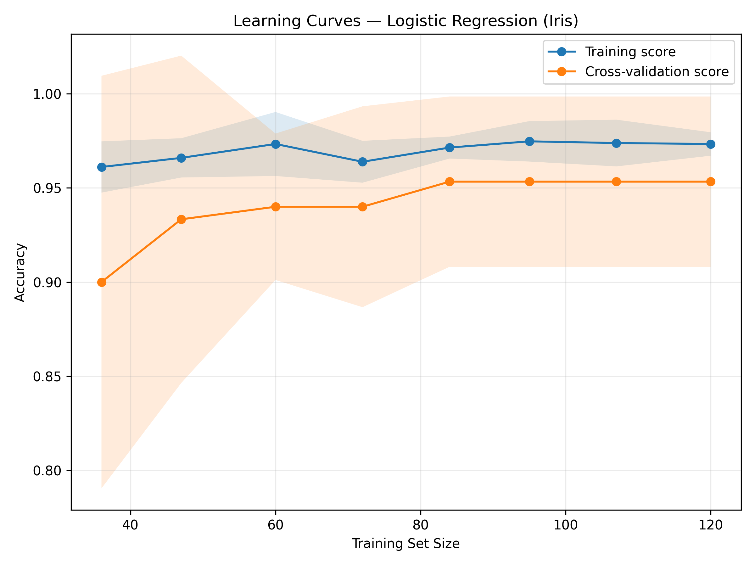
Figure: Learning Curves — Logistic Regression (Iris).
Interpreting the Curves
Learning curves can uncover model behavior patterns:
| Observation | Description |
|---|---|
| Underfitting | Both training and validation accuracy are low and close together. The model is too simple or lacks features. |
| Overfitting | Training accuracy is high but validation accuracy is low, with a large gap. The model is too complex or memorizing the data. |
| Good Fit | Both curves converge at high accuracy, meaning the model generalizes well. |
Key Takeaways
- Learning curves provide a visual diagnostic for model bias and variance.
- Underfitting → Increase model complexity or add more informative features.
- Overfitting → Apply regularization, reduce complexity, or add more data.
- Use StratifiedKFold to ensure balanced evaluation across classes.
- Always analyze learning curves before fine-tuning or deploying your model.
Conclusion
Learning curves are one of the simplest yet most powerful tools in a data scientist’s toolkit.
They don’t just measure performance — they explain it.
By visualizing how accuracy evolves with data, you gain clear insights into your model’s capacity, stability, and generalization.
Use them early in your workflow to save hours of trial and error in model tuning.
Code Snippet:
# Import necessary libraries
import numpy as np
import matplotlib.pyplot as plt
from sklearn.model_selection import learning_curve, StratifiedKFold
from sklearn.pipeline import Pipeline
from sklearn.preprocessing import StandardScaler
from sklearn.linear_model import LogisticRegression
from sklearn.datasets import load_iris


# Load the Iris dataset
data = load_iris()
X, y = data.data, data.target
print("X shape:", X.shape, "| y classes:", np.unique(y))


model = Pipeline(steps=[
    ("scaler", StandardScaler()),
    ("logreg", LogisticRegression(max_iter=1000, multi_class="auto"))
])


cv = StratifiedKFold(n_splits=5, shuffle=True, random_state=42)
train_sizes = np.linspace(0.3, 1.0, 8)  # 30% → 100%, 8 points


sizes, train_scores, test_scores = learning_curve(
    estimator=model,
    X=X,
    y=y,
    cv=cv,
    train_sizes=train_sizes,
    scoring="accuracy",
    n_jobs=-1,
    shuffle=True,
    random_state=42
)

train_mean = train_scores.mean(axis=1)
train_std = train_scores.std(axis=1)
test_mean = test_scores.mean(axis=1)
test_std = test_scores.std(axis=1)


plt.figure(figsize=(8, 6))
plt.plot(sizes, train_mean, "o-", label="Training score")
plt.plot(sizes, test_mean, "o-", label="Cross-validation score")
plt.fill_between(sizes, train_mean - train_std, train_mean + train_std, alpha=0.15)
plt.fill_between(sizes, test_mean - test_std, test_mean + test_std, alpha=0.15)
plt.title("Learning Curves — Logistic Regression (Iris)")
plt.xlabel("Training Set Size")
plt.ylabel("Accuracy")
plt.legend(loc="best")
plt.grid(True, alpha=0.25)
plt.tight_layout()
plt.show()Comments
Add Your Comment
Related Posts

🧩 Python Automation Recipes – 🖥️ System Health Alert

🧠 Python DeepCuts — 💡 Inside Python’s Memory Allocator (pymalloc)

🧩 Python Automation Recipes – 👀 File Change Detector
7-Day AI Crash Course
Learn how AI works, explore real-world examples, and build your first smart models step-by-step.
Perfect for beginners, students, and tech enthusiasts ready to start their AI journey.
No comments yet. Be the first to comment!